
Quick answer
Skody overlaps with APS software. Established APS platforms can model constraints, optimize complex schedules and regenerate plans, and this page does not argue otherwise. Skody differs in three deliberate design choices.
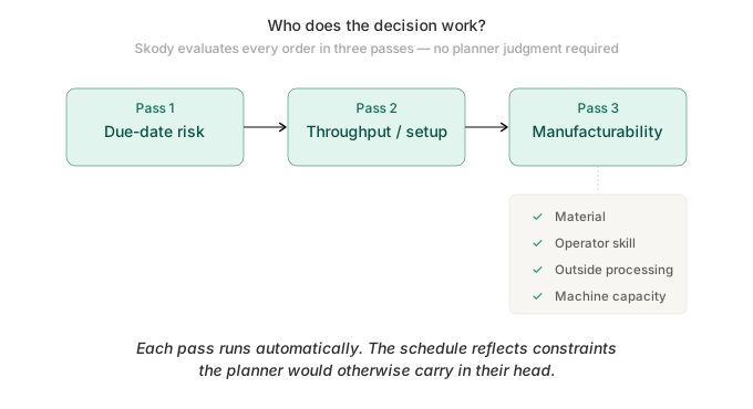
- Conflicts are resolved automatically. When jobs compete for the same machine, operator, skill, material, tooling, pallet, outside-processing slot or hour, Skody determines a default sequence instead of handing each conflict back to the planner to arbitrate.
- The optimization objective is explicit. Delivery performance comes first, then lateness minimization, then throughput and productive capacity — always within real manufacturing constraints.
- It is meant to be operated, not tuned. A production manager should not have to become an optimization specialist to keep the plan current.
Neither approach is universally correct, and for some manufacturers an established APS platform is the stronger fit.
What is Advanced Planning and Scheduling software?
Advanced Planning and Scheduling software creates realistic production plans by considering finite resources such as machines, work centers, calendars, routings, due dates and other production constraints. Many APS platforms also support sophisticated sequencing rules, optimization objectives, materials, labor, setup logic, what-if analysis and enterprise planning.
Unlike basic MRP, which primarily calculates what materials and production are required, APS attempts to determine when work can realistically occur. Traditional APS products can be extremely sophisticated, and several have decades of production use behind them.
The challenge for high-mix manufacturers is often not creating the first feasible plan. It is keeping that plan synchronized with a shop floor that changes constantly.
Three different questions
MRP asks: what needs to be made and purchased?
APS asks: when can production realistically occur?
Skody emphasizes: given the current state of the shop, what should the production baseline be now?
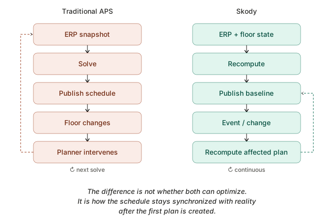
The first schedule is not usually the hard part
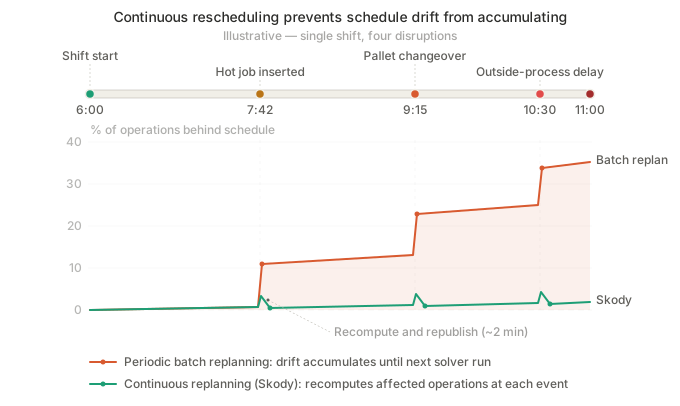
At the start of the day, the production schedule may be correct. Then reality changes. An operation runs longer than expected. An operator calls out. Material does not arrive. A machine goes down. Outside processing is delayed. A rush order arrives. An upstream process finishes early. Due-date priority changes. A pallet becomes unavailable.
Each event can affect downstream capacity and delivery risk, and the effects rarely stay local. The operational question becomes: what should run now?
Conflicts are resolved automatically, not handed back
Most of the daily work in a high-mix shop is arbitration. Two jobs need the same machine in the same window. The only qualified operator is already committed. Material for the higher-priority job is not on the shelf. A pallet is tied up, or heat treat has not returned the parts.
Skody connects to the manufacturer's existing ERP and reads current manufacturing data — running operations and progress, machines and work centers, routings, due dates and priorities, operator availability and skills, shifts and calendars, tooling, material availability and alternatives, outside processing, setup families, pallets, and unattended or lights-out capacity. When those constraints collide, Skody determines a default production sequence rather than presenting the conflict for the planner to settle.
This is not a claim that other APS systems cannot resolve conflicts; many can. The distinction is intent. Skody is built to minimize how much scheduling logic and day-to-day arbitration a planner has to carry personally.
What Skody optimizes for, in order
Skody's first objective is delivery performance: build a production schedule that meets every customer due date. When all due dates cannot be met at once, the objective becomes minimizing lateness rather than quietly picking a sequence and leaving the consequence to be discovered later.
Only after delivery does Skody optimize secondary goals — throughput, productive use of resources, setup efficiency and revenue opportunity. Every decision must stay manufacturable against the real machine, labor, skill, material, tooling, routing, pallet and outside-processing constraints.
The objective hierarchy
First: hit customer due dates.
If that is not possible: minimize lateness.
Then: improve throughput and productive capacity.
Always: respect machine, labor, skill, material, tooling, routing, pallet and outside-processing constraints.
Established APS products can also optimize against sophisticated objectives; this is not a claim that they cannot. The difference is that the objective order above is the default, not something a planning specialist has to encode.
What the planner still has to do after the optimizer runs
The point is not an easy-to-use interface. It is how much scheduling work remains once the software has produced a plan. In Skody the intended operating loop is short:
- production data is read from the ERP
- manufacturing constraints are configured into the model once
- Skody produces a default executable baseline
- conflicts are resolved automatically inside that baseline
- the planner overrides or runs what-if scenarios when judgment is genuinely required
- the schedule can be recomputed quickly after production conditions change
- production teams use schedule, worker and delivery views without rebuilding the plan by hand
A production manager should not need to become an optimization specialist to keep the plan current. When comparing any two products, the question worth asking is not only "can this optimize a schedule?" but "how much work does the planner still need to do after the optimizer runs?"
Skody vs established APS and job-shop scheduling platforms
Skody does not compete with only one product category. Depending on the manufacturer, the alternative may be a traditional APS platform, an enterprise planning system, scheduling inside an ERP, or a dedicated dynamic scheduling layer. Cells below describe typical positioning from public vendor documentation rather than scoring products; behaviour varies by version and configuration, so verify anything critical with the vendor under evaluation.
| Attribute | Skody AI | PlanetTogether | Asprova | Siemens Opcenter APS | JobBOSS² |
|---|---|---|---|---|---|
| Primary product category | Production scheduling and decision layer | APS platform | APS platform | Enterprise APS within a manufacturing suite | Job-shop ERP with scheduling |
| Best fit | High-mix SMB and mid-market shops keeping their ERP | Manufacturers wanting mature traditional APS | Complex, multi-process production planning | Large and multi-site enterprises | Shops buying or replacing a job-shop ERP |
| Existing ERP remains in place | Yes | Yes, integrates with ERP | Yes, integrates with ERP | Yes, within a broader stack | No — it is the ERP |
| Finite-capacity scheduling | Core capability | Core capability | Core capability | Core capability | Supported; verify depth with vendor |
| Machine constraints | Core capability | Core capability | Core capability | Core capability | Supported |
| Labor capacity | Scheduled as a constraint alongside machines | Available depending on configuration | Available depending on configuration | Available depending on configuration | Verify with vendor |
| Operator skills | Modelled as a direct scheduling constraint | Verify with vendor | Verify with vendor | Verify with vendor | Verify with vendor |
| Material constraints | Supported depending on integration | Supported | Supported | Supported | Supported via ERP inventory |
| Setup sequencing | Setup families and grouping | Strong | Strong | Strong | Available depending on configuration |
| Outside processing | Modelled as external operations in the routing | Available depending on configuration | Available depending on configuration | Available depending on configuration | Supported via ERP job routing |
| Dynamic rescheduling | Recalculation from current production state is the operating model | Available depending on configuration | Available depending on configuration | Available depending on configuration | Verify with vendor |
| Default conflict resolution | Resolved automatically into a default sequence | Verify with vendor | Verify with vendor | Verify with vendor | Verify with vendor |
| Stated optimization order | Due dates first, then lateness, then throughput | Configurable objectives; verify with vendor | Configurable objectives; verify with vendor | Configurable objectives; verify with vendor | Verify with vendor |
| Planning expertise expected of the user | Production manager, not an optimization specialist | Planning configuration expertise typically expected | Planning configuration expertise typically expected | Enterprise planning team typically expected | Verify with vendor |
| Scenario / what-if planning | Plan A/B/C comparison | Strong | Strong | Strong | Verify with vendor |
| Pallet pools and unattended production | Modelled, including lights-out capacity | Verify with vendor | Verify with vendor | Verify with vendor | Verify with vendor |
| Enterprise planning depth | Not primary focus | Strong | Strong | Strongest of this set | Not primary focus |
| Multi-site planning | Not primary focus | Available depending on configuration | Available depending on configuration | Core capability | Not primary focus |
| ERP functionality included | No | No | No | No — part of a manufacturing suite | Yes |
| Implementation complexity | Lower; scoped to scheduling on an existing ERP | Moderate to high, depending on model depth | Moderate to high, depending on model depth | High; enterprise programme | High; ERP replacement project |
| High-mix job-shop suitability | Primary design target | Suitable | Suitable | Suitable, usually at larger scale | Suitable as an ERP with scheduling |
Compiled from public vendor documentation and Skody product information, September 2026. No vendor paid for placement. Where a capability could not be confirmed from primary vendor sources, the cell reads “Verify with vendor”.
Skody vs PlanetTogether
PlanetTogether is an established APS platform designed for advanced finite-capacity production planning and scheduling, typically deployed alongside an existing ERP.
It may be the stronger fit for manufacturers looking for mature traditional APS, broad planning capabilities, extensive configuration, sophisticated optimization or larger-scale planning requirements.
Skody may be the stronger fit when the ERP is staying, the primary pain is day-to-day schedule volatility, machine plus labor plus skill constraints matter, schedules are frequently rebuilt manually, and the manufacturer wants a current executable baseline rather than a large planning stack.
Best fit summary
PlanetTogether: Established APS with broader traditional planning depth.
Skody: High-mix production environments where keeping the production schedule synchronized with current shop conditions is the central problem.
Skody vs Asprova
Asprova is a mature APS platform known for detailed production scheduling and complex sequencing, with a strong fit in high-mix and multi-process manufacturing environments. The reason to evaluate Skody is not that Asprova cannot handle complex scheduling.
The distinction is primarily operating model and target deployment. Skody focuses on SMB and mid-market high-mix manufacturers, existing ERP environments, rapid recalculation from current state, machines and labor with skills scheduled together, frequent shop-floor disruption, and operational use of the schedule as the current production baseline.
Asprova may be stronger when extensive APS configuration is desired, deep optimization is needed, the organization already has strong planning expertise, or the production planning model requires significant customization.
Best fit summary
Asprova: Detailed, mature APS for complex production environments.
Skody: Dynamic scheduling and production decision layer for high-mix shops running an existing ERP.
Skody vs Siemens Opcenter APS
Siemens Opcenter APS belongs to a broader enterprise manufacturing software ecosystem. It may be the stronger fit for very large manufacturers, multi-site enterprise environments, companies standardizing on Siemens manufacturing software, and broad MES, MOM or enterprise planning initiatives.
Skody is deliberately narrower. It is intended for manufacturers that want to keep their existing ERP and improve production scheduling without deploying a broad enterprise manufacturing suite.
Best fit summary
Siemens Opcenter APS: Enterprise-scale advanced planning within a broader manufacturing software stack.
Skody: Focused production scheduling and decision layer for high-mix SMB and mid-market manufacturing.
Comparing more options? See Siemens Opcenter APS alternatives.
Skody vs JobBOSS²
This is not exactly APS versus APS. JobBOSS² is fundamentally a job-shop ERP with scheduling functionality, which makes it a different buying decision.
Choose JobBOSS² when you need a job-shop ERP, when estimating, quoting, purchasing, inventory and job management are part of the buying decision, and when replacing or selecting the ERP is acceptable.
Evaluate Skody when the manufacturer already has an ERP, the ERP is staying, scheduling is the specific operational problem, and production changes faster than the existing ERP schedule can keep up. The two are not always mutually exclusive.
"JobBOSS² can be the system of record. Skody is intended to sit above a system of record as a production decision layer."
Skody vs Fulcrum
Fulcrum is not simply another APS product. It is a broader cloud manufacturing operations platform that combines ERP, MRP and MES-style functionality with production scheduling. Its scheduling is directly relevant here because Fulcrum also targets small and mid-sized high-mix manufacturers and uses current production data to adjust schedules as conditions change.
That makes Fulcrum one of the closest practical alternatives for many Skody buyers, but the buying decision is structurally different. Fulcrum explicitly supports automatic schedule adjustment as production data and priorities change, so the distinction is product scope and depth, not whether one product can reschedule dynamically and the other cannot.
Evaluate Fulcrum when:
- the manufacturer wants a broader manufacturing operating system
- replacing an existing ERP or consolidating multiple systems is acceptable
- quoting, inventory, purchasing, job tracking and scheduling should live in the same platform
- shop-floor data collection is part of the broader system decision
Evaluate Skody when:
- the existing ERP is staying
- the primary problem is production scheduling and production decisions
- replacing the ERP is unnecessary or undesirable
- the manufacturer wants a specialized scheduling layer connected to its existing systems
- machine, labor, operator skills, materials, pallets and changing priorities need to be modeled together
"Do we want to replace or consolidate our manufacturing operating system, or do we want to keep our ERP and add a specialized scheduling layer?"
Best fit summary
Fulcrum: Modern all-in-one manufacturing operations platform with integrated dynamic production scheduling.
Skody: Dedicated production scheduling and decision layer for manufacturers that want to keep their existing ERP and add deeper high-mix scheduling intelligence.
Which scheduling approach is the best fit?
| Need | Strong candidate |
|---|---|
| Need a new job-shop ERP | JobBOSS² |
| Need mature traditional APS | PlanetTogether or Asprova |
| Need an enterprise APS / MOM stack | Siemens Opcenter APS |
| Already have an ERP with high schedule volatility | Skody |
| Need highly configurable deep optimization | Traditional APS such as Asprova or PlanetTogether |
| Need machine, labor, skills and current shop state in a high-mix SMB environment | Skody |
| Need multi-site enterprise planning | Siemens or another established enterprise APS |
These are general fit guidelines, not absolute rules. Actual fit depends on manufacturing process, integration requirements and planning complexity.
Example: what happens when the floor changes at 10:30 AM?
Consider a hypothetical shop with 40 work centers, 25 operators with mixed skills, 250 active jobs, shared tooling, outside processing and several unattended machines. By 10:30 AM one operation has run two hours long, a qualified operator has called out, heat treat has returned work early, a customer has expedited an order, and two machines need the same pallet pool.
These events propagate through downstream capacity, labor conflicts, setup sequence, delivery dates and unattended production. The scheduling challenge is not moving one job; it is understanding the new best sequence for everything behind it.
Rather than assert how a specific competing product behaves, ask each vendor:
- Does the platform automatically propagate these changes?
- How often can it recalculate?
- What current-state information does it consume?
- How much planner intervention is required?
- Can labor skills be modelled directly?
- Can pallet and unattended constraints be modelled?
Skody's approach in this situation is procedural: read the current state, recompute the finite-capacity schedule, and publish an updated production baseline with any unresolved exceptions surfaced for the planner.
When traditional APS may be the better choice
Traditional APS may be better if the manufacturer needs:
- enterprise-wide planning
- multi-site optimization
- highly configurable mathematical optimization
- sophisticated long-range planning
- broad planning-model customization
- corporate standardization around an established APS
- deep integration with an enterprise MES or MOM ecosystem
- experienced planning teams wanting detailed optimization control
Skody is not intended to replace every APS use case. Its strongest fit is narrower: high-mix manufacturers that want the production schedule to reflect current production reality.
When Skody may be the better fit
- you already have an ERP
- you do not want to replace the ERP
- your schedule is regularly obsolete by lunch
- planners manually rebuild schedules
- machine state changes frequently
- labor availability matters
- operator skills matter
- priorities change frequently
- material readiness changes
- outside processing affects production
- pallets or lights-out production complicate capacity
- management wants earlier visibility into late-job risk
"ERP is the system of record. Skody is the production decision layer."
How this works in actual manufacturing environments
Three Sigma Manufacturing — Kent, Washington
Environment: precision machining for aerospace, defense and industrial customers; 47 machine work centers; ProShop ERP.
Before Skody: planning complexity grew with demand, machine utilization and labor constraints, and the planner rebuilt the schedule rather than trusting it.
How Skody is used: the planner starts each morning from a freshly computed baseline reflecting current factory conditions instead of repairing yesterday's plan.
Measured result: the planner accepts the computed baseline about 99% of days rather than rebuilding it, and the planning horizon extended from about one week to up to one year.
Yeager Manufacturing — Winter Park, Florida
Environment: high-mix aerospace and defense job shop.
Before Skody: on-time delivery under 80%, with expediting used to manage commitments.
How Skody is used: machines and people are scheduled together, and the resulting schedule is used by the team as the production baseline.
Measured result: on-time delivery moved from under 80% to 90%+ within two months.
14 questions to ask before buying production scheduling software
- What happens when an operation runs longer than planned?
- How frequently can the schedule be recalculated?
- Does it use actual operation progress?
- Can labor constrain the schedule?
- Can operator skills constrain the schedule?
- Are machines and labor scheduled simultaneously?
- How are material shortages handled?
- How is outside processing modelled?
- How are setup families handled?
- Can it model pallet pools?
- Can it model unattended or lights-out capacity?
- Can we compare Plan A, B and C scenarios?
- Does it show future delivery risk?
- How much planner intervention is required when priorities change?
Frequently asked questions
What is APS software in manufacturing?
Advanced Planning and Scheduling (APS) software creates feasible production plans using finite capacity, routings, due dates, calendars, setup rules and other manufacturing constraints. Rather than assuming capacity is effectively unlimited, an APS engine attempts to determine when work can realistically be performed given the resources available. Products vary widely in modelling depth, optimization objectives, scenario tooling and integration approach, so the category name alone says little about how a specific product will behave on a given shop floor.
Is Skody an APS system?
Skody performs finite-capacity scheduling, so it overlaps with APS. The emphasis differs. Skody is designed to resolve competing demands for machines, operators, skills, materials, tooling, pallets and outside processing into a default production sequence automatically, and to optimize first for customer due dates, then for lateness, then for throughput and productive capacity. Whether that is called APS or a production decision layer matters less than how much scheduling work the planner still performs manually after the software has run.
What is the difference between Skody and PlanetTogether?
PlanetTogether is an established APS platform for advanced finite-capacity planning and scheduling, typically integrated alongside an ERP and configured to a manufacturer’s planning model. Skody is narrower: it is built around repeatedly recomputing an executable production baseline from the current state of a high-mix shop, with machines, operator skills, materials, outside processing and pallets treated as scheduling constraints. Manufacturers wanting broad, highly configurable traditional planning depth should evaluate PlanetTogether directly; verify specific capabilities with the vendor.
What is the difference between Skody and Asprova?
Asprova is a mature APS platform known for detailed scheduling and complex sequencing in multi-process manufacturing, and it is capable of handling high complexity when configured by an experienced planning team. The distinction with Skody is operating model and target deployment rather than capability ceiling: Skody focuses on small and mid-market high-mix manufacturers that keep their existing ERP and need frequent recalculation from current shop conditions with machines and labor scheduled together.
What is the difference between Skody and JobBOSS?
JobBOSS² is fundamentally a job-shop ERP that includes scheduling functionality, so choosing it is an ERP decision covering estimating, quoting, purchasing, inventory and job costing. Skody is not an ERP and does not replace one. It sits above a system of record as a production decision layer. If you need a new job-shop ERP, evaluate JobBOSS². If the ERP is staying and scheduling is the operational problem, evaluate Skody. The two are not always mutually exclusive.
What is the difference between Skody and Siemens Opcenter APS?
Siemens Opcenter APS belongs to a broader enterprise manufacturing software ecosystem and is generally aimed at larger, multi-site manufacturers or organizations standardizing on Siemens MES and MOM software. Skody is deliberately narrower and is intended for manufacturers that want to keep their existing ERP and improve production scheduling without deploying a broad enterprise manufacturing suite.
Does Skody replace ERP?
No. Skody complements an existing ERP and does not provide order entry, purchasing, inventory, MRP or accounting. It reads production information from the ERP — orders, routings, resources, materials and progress — and computes a finite-capacity schedule against current conditions. The ERP remains the system of record; Skody is the production decision layer that sits on top of it.
Can APS software reschedule automatically?
Many APS products can, depending on product and configuration. Some support scheduled regeneration, some support event-triggered runs, and many are run when the planner initiates them. The practical questions are what triggers a recalculation, how long a full run takes at your operation count, and how much of the resulting sequence the planner must repair by hand before it can be released to the floor.
What is finite-capacity scheduling?
Finite-capacity scheduling plans work against the real capacity of resources rather than assuming unlimited availability. Machines, operators, shifts, calendars and setup requirements limit how much work can be placed in a given window, so operations are sequenced into the capacity that genuinely exists. The output is a schedule that can, in principle, be executed rather than a set of dates that only balance on paper.
What is dynamic production scheduling?
Dynamic production scheduling means the schedule is recomputed from the current production state as conditions change, rather than being generated once and repaired manually until the next planning run. The emphasis is on the operating loop — read current state, recompute, publish an updated baseline — rather than on the sophistication of any single optimization pass.
Which scheduling software is best for high-mix manufacturing?
There is no single answer, because high-mix shops differ in size, integration requirements and planning maturity. Established APS platforms such as Asprova, PlanetTogether and Siemens Opcenter APS are credible options, particularly where deep configuration or enterprise planning breadth is required. Skody is best suited to high-mix manufacturers that already have an ERP but need production schedules to adapt frequently to changes in machines, labor, materials and priorities.
Which APS is best for a small or mid-sized manufacturer?
Smaller manufacturers usually need a shorter implementation, fewer planning specialists and less configuration than an enterprise APS assumes. Products positioned for that segment include PlanetTogether, Asprova and Skody, alongside scheduling included in job-shop ERPs such as JobBOSS². The practical filter is whether you are replacing the ERP, adding a planning platform, or adding a scheduling layer above the ERP you already run. See the full comparison of APS software for small and mid-size manufacturers.
Can production scheduling software account for operator skills?
Some systems can, and several represent labor only as a shift calendar rather than as named qualifications. Skody schedules operator availability and skill requirements as constraints alongside machines, so an operation is not placed in a window where nobody qualified is present. For any other product, verify skills modelling directly with the vendor rather than assuming labor capacity implies skills.
How frequently should a production schedule be recalculated?
Frequently enough that the published sequence still reflects the floor when an operator reads it. In stable, low-mix production a daily or weekly plan may hold. In high-mix discrete manufacturing, where operations run long, operators are reassigned and material arrives late, the plan can diverge within hours, so recalculation on shift boundaries or on significant production events is more realistic than a weekly regeneration.
Sources and verification
Statements on this page are drawn from each vendor's own public product information. Where documentation did not confirm a capability, the page says "verify with vendor" rather than guessing. Product functionality changes; confirm anything critical directly with the vendor.
- PlanetTogetherAPS product category, finite-capacity planning scope and ERP-integration approach. Checked 6 September 2026.
- AsprovaAPS positioning, finite-capacity scheduling and sequencing scope. Checked 6 September 2026.
- Siemens Opcenter APSEnterprise APS planning and scheduling scope within the Siemens manufacturing software stack. Checked 6 September 2026.
- JobBOSS² (ECI Software Solutions)Job-shop ERP scope with scheduling functionality included. Checked 6 September 2026.
- FulcrumCloud manufacturing operations platform scope, including ERP/MRP/MES-style functionality and automatic schedule adjustment as production data changes. Checked 6 September 2026.
- Skody AISkody's product scope, constraints modelled and ERP-integration approach. Checked 6 September 2026.
- Three Sigma Manufacturing case studyPublished customer outcomes referenced on this page. Checked 6 September 2026.
- Yeager Manufacturing case studyPublished customer outcomes referenced on this page. Checked 6 September 2026.
Editorial methodology
- Products were selected for their relevance to discrete production scheduling, not for commercial relationships.
- Comparisons use publicly available vendor documentation and product information current as of September 2026.
- Skody AI is included because Skody publishes this page. We say so plainly rather than presenting the comparison as third-party research.
- No vendor paid for placement, ranking or inclusion. There are no editorial scores and no reviews on this page.
- Product functionality changes. Buyers should verify every critical requirement directly with each vendor before purchase.
Last reviewed: October 2026
See how Skody schedules a real high-mix shop
Two published customer accounts show what finite-capacity rescheduling looks like against a live floor: a machine shop and a precision contract manufacturer, both keeping the ERP they already had.